No significant difference? Oh really? How to recognize weaknesses in muscle hypertrophy studies.

Congrats!

You’re hired.

As a PhD student in muscle metabolism.

You want to determine what’s the best moment to eat protein for muscle mass gains.

Morning or evening? Sounds easy enough, right? Just do a study where one group gets protein in the morning, and the other group gets it in the evening, and see which group comes out on top.

Unfortunately, it’s a bit more complicated than that.

Let me explain why.

You have to take the power of the study in consideration.

What kind of power? Statistical power.

Still here?

Good! Because a proper understanding of statistical power is a research superpower.

Unfortunately, most people don’t really understand it or are even aware of the concept. However, understanding statistical power is essential to properly read and evaluate research.

Don’t worry, this won’t be boring statistics lecture with a lot of confusing numbers and formulas. Instead, we’ll give practical examples of the factors that influence statistical power and how these impact the interpretation of muscle growth (muscle hypertrophy) research.

If you just want the main message, see this video:

This article is written as a kind of comprehensive wiki. Ideally, you take the time to read everything from A to Z to let the content sink in. However, you can just jump to a specific section of interest by clicking the links in the table of contents below. You can also just scroll to the figures and read the highlighted main points.

Heck here is a short summary:

Note that the figures are fictive data to illustrate how various research designs impact statistical power.

Footnotes are inserted to provide more details that are not interesting to most people such as technical definitions.

1I’m a footnote, I’m usually boring. I’m here for technical disclaimers so statisticians don’t get upset.

ghghgh

1. Statistical power

This section is the most boring, because it explains the basic principles of statistical conclusions (don’t worry, it will get much better after this).

If the figure below makes sense to you, you can skip this section altogether and jump to section 2 where we link this to muscle hypertrophy research.

If the picture above makes sense to you, please skip ahead to section 2 where we link these concepts to muscle hypertrophy research. If the picture isn’t entirely clear, this section will help you.2Be aware this section can be boring because it explains basic statistical concepts. It’s just something you have to get through, the other sections will use practical muscle hypertrophy examples.

A research study can be compared with a pregnancy test.

A good pregnancy test indicates you’re pregnant when you’re actually pregnant. And it indicates you’re NOT pregnant when you’re in fact NOT pregnant (so the the conclusion from the test reflects reality).

If you found out your pregnancy test gave you a wrong conclusion, you won’t be very happy.

It’s the same thing with research studies. You want the conclusion of a research study to be the correct conclusion in reality.

Unfortunately, conclusions for research studies are not correct 100% of the time.

For example, you can never say with 100% certainty that you would get the exact same result or conclusion if you took a different group of subjects.

Just as with a pregnancy test, there are two different types of wrong conclusions a research study can make.3…at least when using traditional null-hypothesis significance testing.

The first type of wrong conclusion is called a false positive result (type 1 error). The test indicates a significant result, but this is not true in reality. For example, the test indicates you’re pregnant when you’re not.

The second type of wrong conclusion is called a false negative result (type 2 error). The test indicates no significant result, but in reality, there’s actually a significant difference. For example, the test indicates you’re NOT pregnant when you actually are pregnant.

The chance of making a type 1 error is related to the p-value. The p-value is usually set at 0.05. This means that statisticians have agreed that a 5% chance of making this type of error is acceptable.

Therefore, a pregnancy test that has a 5% chance or less to say you’re pregnant when you’re not would be considered an acceptable test in research (keep it mind it’s impossible for a research test to be correct a 100% of the time). 4Although there are usually much lower error rates allowed when a false positive can have a major impact such as when you test false positive for cancer and therefore have to receive dangerous treatments.

The chance of making a type 2 error is related to statistical power. The higher the statistical power, the lower the chance of making this type of error. A statistical power of at least 80% is considered to be acceptable. However, this means there is still a 20% chance you make a type 2 error (100 minus the power = 20).

Therefore, a pregnancy test that has a 20% chance or less to indicate you’re NOT pregnant when you actually are would be considered an acceptable test in research.

This number might seem quite high to you, but it’s often even worse than that in research.

However, the prevention of this type of error (type 2 error) gets relatively little attention. For example, it is rare that statistical power even gets reported. And after reading this article you will realize that many muscle hypertrophy studies don’t even come close to a statistical power of 80%.

This means that a lot of studies report no significant difference in muscle hypertrophy between treatments when in reality one of the treatments is superior to the other.

The power of a study depends largely on the research design. This includes factors such as study duration, number of subjects, and which muscle mass measurements are made.

We’ll break down the impact of all these factors on statistical power and will give practical and understandable examples for each. By the end of this article, you’ll realize why understanding these concepts is essential to make proper conclusions from research.

2. Determinants of statistical power

2.1 Study duration: muscle hypertrophy is a slow process

We have all seen the bold claims: gain 25 pounds of muscle in just 8 weeks!

Unfortunately, muscle hypertrophy is a slow process. Some people simply don’t want to believe it and convince themselves that their weight gain during a bulk is ‘’mostly muscle’’.

But when we measure muscle mass gains in the lab with the most sophisticated techniques, we don’t see gains anywhere near the internet claims. And I’ve seen more people throw up in labs than in gyms, so it’s not because subjects in research don’t train hard enough.

In fact, it takes several weeks of training before we can even detect a statistically significant increase in muscle mass.

This figure above illustrates that it takes some time before you can detect a significant difference in muscle mass between two groups. For example, training for 3 weeks would result in a slight increase in muscle mass compared to a control group (illustrated by the red line in the red area). However, this difference is too small to be considered statistically significant. Therefore, a 3-week study would conclude that resistance exercise does not increase muscle mass, while in reality, it does.

In other words, a 3-week study would be underpowered and draw a wrong conclusion.

The green line represents the study duration from which on the difference between the groups would be big enough to be statistically significant. In other words, it would take at least a six-week study to have a good chance (~80%) to show that resistance training significantly increases muscle mass in this example. If the study runs even longer, the chance on statistically significant results increases even further.

In other words, a longer study duration increases the statistical power.

(Reminder: The statistical power of a study depends on a lot more factors than just its duration, as will be discussed in the sections below. Therefore, you can’t say that a study is underpowered by only looking at its duration. A study shorter than 6 weeks CAN be sufficiently powered depending on its other factors).

2.2 Study duration vs difference between groups

The example in the previous section was quite extreme.

You would expect a pretty big difference in muscle mass gains between a group that trains compared to a group that doesn’t train.

But what if the difference between the groups is less extreme?

Let’s compare two training protocols instead of comparing training vs non-training. Imagine one group doing 3 sets per muscle group each training session and the other doing 1 set per muscle group each session.

Again, the green bar indicates the earliest time point where there is a significant difference between the two groups. The length of the green bar is also the same as in the previous example, representing the same difference between the two groups that is required for statistical significance. This green bar has moved to the right in this example: it now takes 12 weeks instead of 6 weeks to get this difference between groups.

This demonstrates that the difference between groups required for statistical significance not only depends on study duration, but also on which comparison you’re making.

In the previous section, you saw that a big difference between groups (training vs non-training) requires only a short study period (6 weeks). In this section, the difference between groups is smaller (3 sets vs 1 set), and therefore you need a longer study duration to compensate.

In other words, the smaller the difference between groups, the longer the study duration has to have sufficient statistical power.

2.3 Study duration: the law of diminishing returns

In figure 3 in the previous section, we saw that doing three times as much work (3 sets vs 1 set) resulted in only 50% more gains. This is what we typically see: relatively little effort gives most of the results. More effort produces relatively small additional results.

The bang-for-your-buck decreases.

The law of diminishing returns dictates that performing 3 sets does not produce 3 times the results that 1 set produces. However, 1 and 3 sets are both relatively little. They are still on the left part of the curve where each additional set produces a relatively large increase in results.

What if you’re interested in 6 sets vs 7 sets?

Not only is the difference between the groups only 1 set. The 6 sets group is already doing 6 sets, so the additional value of 1 set is very little. The additional value of 1 set depends on how much you are already doing.

In the figure above you can see that the 7 set group gains slightly more muscle than the 6 set group. However, the difference between the groups is so small, that is doesn’t result in statistical significance. Therefore, this study would conclude there’s no significant difference between the groups, even though in reality 7 sets is slightly better than 6 sets.

In other words, this study would be underpowered.

It’s relatively easy to get a significant difference in muscle mass gains when you compare one group that trains very well to another group that trains suboptimal. However, when comparing two groups that are both training quite effectively, the difference between them is going to be small. Therefore, it’s very difficult to find a significant difference between two groups that both train effectively.

However, the absence of a statistically significant difference between groups should not be confused with the conclusion that ‘’both groups had the same result’’.

5Such a conclusion requires other approaches such as equivalence testing. For details: Equivalence Testing for Psychological Research: A Tutorial

Such studies are just underpowered to make the correct conclusion.

2.4 Variation

Up to this point, we’ve acted like training results in a fixed amount of muscle mass gains. Train for 6 weeks and you gain 0.9 kg of muscle mass. Train for 12 weeks and you gain 1.7 kg of muscle mass.

In practice, muscle mass gains aren’t that straightforward. There is a huge variation in the amount of muscle mass that different subjects gain.

Before we discuss the causes of these individual responses, let’s first discuss the impact of variation on statistical power.

Let’s say that we do a small study with 6 subjects doing training program X, and 6 different subjects doing training program Y.

Figure 6A shows that subjects in training program Y gained on average more muscle mass than subjects on training program X (1.5 vs 1.0 kg). However, there is quite some variation between the subjects. Several subjects on training program X gained more muscle mass than some of the subjects on training program Y.

It is hard to be certain that training program Y is really better than training program X due to the variation. Maybe the subjects on training program Y gained more on average because they had better genetics, or they slept better, or ate more protein for example. You would expect most subjects on training program Y to gain more than subjects on training program X is training Y was so much better.

In figure 6B, the average gain in training program X and Y are the same as in figure 6A (again 1.5 vs 1.0 kg). However, it’s quite easy to see that program Y is superior to program A because of the low variation (almost every dot is higher in program Y compared to X).

Above, we looked at variation and took this into account to draw our conclusions. Statistical tests do the same thing (except they use accurate formulas for this purpose).

Statistical tests are much more likely to conclude that there is a statistical significant difference when there is little variation.

2.4.1 Variation: differences between subjects

The first factor that contributes to variation is genetic differences between subjects.

If I do training program A and gain more muscle mass than you gain on training program B, are you completely convinced that my training program is better?

I hope not.

It could simply be that I have better genetics and would gain more muscle mass than you even if we switched programs.

Another explanation why I might have gained more than you could be that my lifestyle factors are much better than yours. For example, I might sleep an hour longer than you each day, have a much better diet, a lot less stress, etc.

Therefore, it would be difficult to conclude that my training program is the reason I made better muscle mass gains than you.

So how we reduce the impact of factors such as genetics and lifestyle in a research study?

The first thing we can do is to increase the number of subjects.

Instead of comparing the two of us, we could compare two groups of subjects. For example, if 6 subjects are on training program A and gain significantly more muscle mass than 6 subjects on training program B, that would already be more convincing than just comparing you vs me. However, you could still make a reasonable case that maybe the 6 guys in each group are not necessarily reflective of everyone, and if you would run the experiment again with another 6 subjects, the results would be different.

However, you have much less reason to doubt the data if 100 subjects on training program A gain significantly more muscle mass than subjects on training program B. The average characteristics of the groups are usually the same when you have a large sample size: a similar number of genetic freaks, similar number of poor sleepers etc.

Why is that?

Let me explain by using the analogy of flipping a coin.

You expect heads 50% of the time when flipping a coin. But it’s definitely possible to get tails 5 times in a row (unlucky, but possible). However, the average amount of heads will be very close to 50% if you flip the coin a thousand times. Because of the large number of flips, any unlucky streak of tails will eventually be balanced with a lucky streak of heads.

It’s the same with selecting subjects in a study. With a low number of subjects, you might be unlucky and include a couple of genetic freaks which will drastically influence the group average. But the more subjects you include, the more likely that your group reflects the true average.

Therefore, you are more confident in your data and more likely to draw the right conclusion with a high number of subjects.

2.4.2 Variation: within-subject comparison

In the previous section, we discussed how differences between subjects make it difficult to draw strong conclusions. Therefore, you need to compensate with a high number of subjects to get sufficient statistical power.

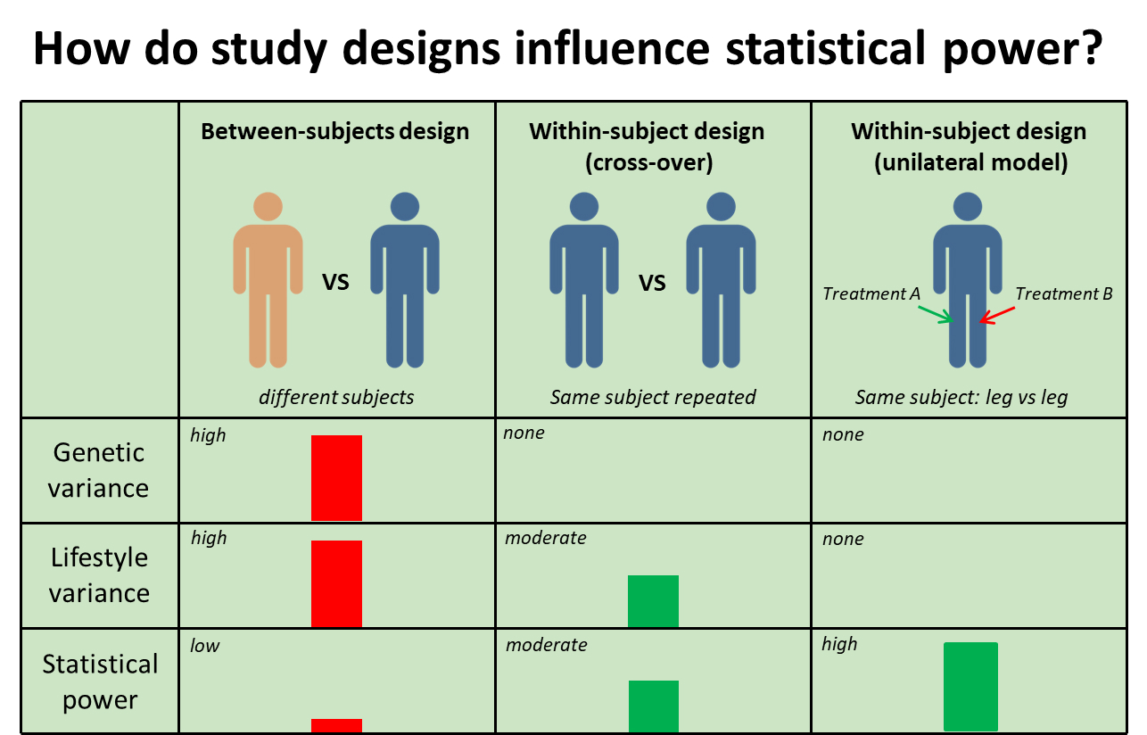
Another option is to test different training programs in the same subject. For example, a subject would perform both training program A and training program B.

This is called a within-subject design.

The biggest advantage of this approach is that you eliminate genetic differences, because you compare both training programs in the same subject. Therefore, you’re more convinced that a difference in gains between the two programs is the result of the programs.

An example of this is a cross-over design. The subject first does training program A, then training program B for example.

However, there are some limitations to a cross-over design with strength training studies. The first is that there’s likely a carry-over effect. If you would start another program right away, you’re going to make worse gains because of the law of diminishing returns.

Of course, you can wait for some time before starting the second training program to lose all your gains, which is called a wash out period. However, it’s still easier to regain muscle mass and strength once you’ve had it before (called muscle memory) (Seaborne et al., 2018).

Therefore, these designs have the benefit of eliminating genetic variation and lowering lifestyle variations (e.g. how much you sleep is probably relatively similar during both periods), but they are not perfect.

Another variant of a within-subject design is the contralateral model.

For example, your left leg performs training program A while your right leg performs training program B. This way you don’t have the genetic differences, you don’t have the muscle memory problem, and the differences in lifestyle factors are completely eliminated as well (e.g. the amount of sleep you have is by definition the same for each leg).

Therefore, a contralateral model results in more statistical power compared to a cross-overdesign, and both are superior to a between-subject design (different people in different groups).

There are two drawbacks of a contralateral design.

The first is that training your one leg might have some impact on your other leg, and vice versa. This would reduce the difference between legs. The other potential drawback is that nobody trains exclusively single legged, thereby reducing external validity (how reflective the results are of the real world). However, the latter shouldn’t matter much as studies are mostly interested in principles (e.g. is high volume better than low volume).

These drawbacks are often much less important than the benefits this design has for statistical power.

2.4.3 Variation: Measurement error

Another factor that contributes to variation is measurement error. No measurement is perfect, there’s always some error.

You can try to use a tape to measure arm circumference as an indicator of muscle mass. However, it is unlikely that you always do the measurement perfectly the same, no matter how good you try to standardize it. For example, arm circumference can be influenced by a slight shift in the location of the measurement, the angle of the tape, or how hard you pull the tape.

Those are examples of human errors. The tape itself has no variation: an inch is an inch. In contrast, machines always have some measurement variations.

For example, a DEXA makes a whole-body scan and measures bone mass, fat mass and lean body mass. However, you won’t get exactly the same values if you perform multiple DEXA scans right after each other.

Imagine taking three DEXA scans right after each other and the 3 scans show that you have 40, 42, and 41 kg lean mass. Seems pretty close right?

You start with a new 6-week training program, after which you do a final DEXA scan to evaluate your progress.

The DEXA scan shows 42 kg lean mass this time. So what happened?
• Did you gain 2 kg compared to the 40 kg lean mass scan of last time?
• Did you stay the same compared to the 42 kg scan of last time?
• Did you gain 1 kg compared to 41 kg (the average of last time)?

You can’t really be sure, can you?

Now, imagine the 3 measurements the first time were 40.9, 41.1 and 41.0 kg (same 41 kg average, just a lot less variation). A final scan of 42 kg now seems to indicate a clear improvement.

This illustrates how measurement error makes it harder to draw a conclusion.

There are several ways to illustrate variation in research. A common method is to show standard deviation bars above and below an average. The smaller these bars, the smaller the variation.

Using a poor method to assess muscle mass gains is not an issue when you expect a big difference between the groups. But you should use the best methodology if you expect a small difference between groups to have a shot at finding statistically significant differences.

You should always consider which measurement tool and techniques were used in a study. How prone is it to human error, how big is the technical error, etc.

Another consideration is what your method really measures. For example, a tape measure doesn’t really measure muscle mass, it’s also influenced by changes in fat mass.

Poor methods reduce the power of the study. Cross-sectional area as measured by CT, MRI, or muscle fiber histology are considered strong measurements.

2.5 Training status

Studies with trained subjects are often well-received on social media by evidence-based fitness enthusiasts (which are obviously relatively trained themselves). It is typically regarded as a strong point of a study.

It is often said that ‘everything works’ in untrained subjects, and therefore studies in untrained subjects are supposed to have little value.

Let me explain why this makes little sense.

This argument would make sense if untrained subjects made maximal muscle gains even with suboptimal training programs. Because they would gain just as much with a suboptimal training program as with a much better training program. Therefore, the study would conclude there is no difference between the programs, when in reality the programs aren’t the same (or at least not the same for all populations).

However, that is not the case. Suboptimal training programs produce suboptimal muscle mass gains in untrained subjects (e.g. 1 set produces worse results than 3 sets: (Mitchell et al., 2012). Therefore, a study with untrained subjects would draw the correct conclusion that better training programs are indeed better.

In fact, studies with trained subjects can have a pretty big drawback.

Take one guess?

You got it. Low statistical power.

Let me explain why.

Remember the law of diminishing returns? Muscle mass gains are a nice example of diminishing returns. You make rapid muscle mass gains when you begin lifting, but gains slow down rapidly as you’re getting more trained.

So why does this matter?

The more trained subjects are, the more difficult it is to make muscle mass gains. Very highly trained subjects will make little to no muscle mass gains even during a few months of training.

When neither training program results in measurable muscle mass gains, it’s of course not possible to see differences between the programs.

In the figure above, you would have to conclude that training program B is not significantly better than training program A based on the statistics. But if you just look at the statistics, then you would also have to conclude that training in general is not effective to increase muscle mass in trained subjects (that conclusion is simply not correct).

The rate of muscle mass gains is so slow in trained subjects that it’s much harder to obtain statistically significant findings.

Figure B has zoomed in on the results. It appears that both groups are gaining a very small amount of muscle and training program B gains just a bit more than training program A. However, the increase in muscle mass is miniscule compared to the variation. Simply said, we don’t have machines that can detect such small increases in muscle mass; their measurement error is too big.

Therefore, trained subjects lower the power of your study.

Don’t get me wrong, this does not mean that doing studies in trained subjects is always a poor choice. It’s pretty impressive if you do get statistically significant differences in trained subjects. It means one training program is much better than the other and/or that you had a very big study (long duration, many subjects etc), otherwise you would not reach statistical significance.

However, you’ll always wonder if there’s truly no effect or that a study was simply underpowered when no statistical significant differences are observed in trained subjects. Therefore, it is very hard to conclude that something ‘’doesn’t work’’ in trained subjects. A small improvement in performance or muscle mass might be worth a lot in competing athletes, but is almost impossible to detect in a study.

2.6 Multiple comparisons: are more groups better?

Imagine a simple study that compared the effect of 3 sets per exercise vs 9 sets per exercise on muscle mass gains. The results indicate that the 9 sets per exercise protocol resulted in 3 times as much muscle mass gains. See Figure A below. You’re likely left with a lot of questions after reading this study.

For example, what would happen with a 6 set per exercise protocol? You might expect the muscle mass gains of 6 sets to be right in between those of the 3 sets and 9 sets protocols.

However, remember the law of diminishing returns? You cannot assume that gains are linear. Therefore, it might be that 6 sets give almost the same result as 9 sets. You can even speculate that 6 sets are optimal and would give better gains, because 9 sets may results in overtraining. You could also argue that you need a minimal dose of volume, before growth really kicks in (see figure B).

Therefore, adding an extra group to this study would give you a much better understanding of the dose-response relationship between the number of sets per exercise and muscle mass gains.

However, an obvious problem is that adding another group would require 50% more work, money and willing subjects (an increase from 2 to 3 groups).

The impact on statistical power may be less obvious.

There is only one comparison when there are two groups: 3 vs 9 sets.

There are 3 comparisons when there are 3 groups:
– 3 set vs 6
– 3 set vs 9
– 6 sets vs 9

Therefore, you would run 3 statistical comparisons instead of just 1.

Remember the pregnancy test at the beginning of the article? It could give you the wrong conclusion that you are pregnant when you are not. It’s a small chance, but it can happen.

But what if you would keep doing more and more pregnancy tests? Sooner or later, one of them is going to give you the false result that you are pregnant.

The same thing happens with statistical tests.

Scientists have agreed that it’s ok that tests have a 5% chance of giving a false positive result (e.g. a pregnancy test that would claim you’re pregnant while you’re not). This is related to a p-value of 0.05 that you often see mentioned in papers.

This mean that on average for every 20 tests you do, one of them gives you a false positive result (20 x 5% = 100%).6The formula for determining the new error rate for multiple t-tests is not as simple as multiplying 5% by the number of tests. However, if you’re running a few tests, the results are very similair. For example, three t-tests would be 15% (actually 14.3%). The increase in error rate with doing multiple t-tests is called famillywise or experiment wise error rate.

This may sound like a high number to you. Why do scientists not have stricter criteria for the p-value so there would be less false positive findings?

The stricter your criteria are, the lower your statistical power is.

You essentially become a sceptic with stricter criteria (e.g. a p-value of 0.01 instead of 0.05) Even when research data seems to suggest that one group is clearly better than another, you just say ‘’I’m not convinced’’. This would result in many conclusions that there is no ‘’statistically significant’’ difference, when in reality there is a difference (in other words, you lower the power of a study).

Therefore, we have a problem. We get false positive results if we run too many tests, but we would often reject real differences when we are extremely skeptical.

The solution is to base your amount of skepticism on the number of tests you do.

A p-value of 0.05 is good if you run one statistical test (one comparison). But you have to become more skeptical of each tests when you make more comparisons.

The most common approach is a post-hoc Bonferonni correction. It divides the p-value by the number of tests you do. So, in the case of 3 comparisons, results would only be considered significant when the p-value is 0.05/3 = 0.016 or lower.

Therefore, adding one group makes it much harder to get statistical significance on any of the comparisons in the study. In other words, the statistical power went down dramatically.

How could you compensate for this?

More subjects, longer duration, more sensitive measurements etc.

Therefore, the addition of one group doesn’t require just 50% more work, money, and willing subjects. It requires MUCH more work, money and willing subjects to also compensate for the much lower statistical power and to have a realistic shot at statistically significant results.

It’s often not a good idea to include multiple groups in a muscle hypertrophy study. Low statistical power is already an issue for many research questions. Adding more groups makes it disproportionally more difficult to get statistical significance. It’s often much better to use all your resources to just make one comparison.

3 Consequence of low statistical power

A study with low statistical power is essentially doomed before it ever began. It has little chance to conclude there is a statistically significant difference between the groups. The problem of this is that it will result in a paper that gives the wrong conclusion. For example, you conclude there is no difference between 4 sets or 6 sets per body part, while in reality 6 sets is better, but you simply had too little statistical power in your study. Most people don’t have the statistical expertise to recognize this and just go by the title and abstract of the study.

Before you can run a study, you need approval from an ethics committee. A good ethics committee would not even allow an underpowered study because it would only result in a study that would likely give a wrong message to the world. But often the quality of the ethics committees goes hand in hand with the resources of the university.

So the labs who have the resources to run big studies with sufficient statistical power are connected to ethical committees who understand statistical power and would be very strict. In contrast, labs with less financial means also tend to have less qualified ethical committee or committee that simply approve studies even when they know they have little statistical power simply because that is all what the resources allow. In that case, it is very important that the researchers at least are aware of the limitation and mention it in their study.

Keep in mind that an underpowered study does not prove that there is no difference between two treatment or that a treatment ‘’doesn’t work’’. In fact, it doesn’t really prove anything but creates a lot of uncertainty and sets a lot of people on the wrong foot. However, the study can still be valuable, as we’ll discuss later.

4 Two examples why power is so important

So far, we have discussed how various factors such as study duration and sample size impact the power of a study. Now let’s have a look at some research and whether it is properly powered.

4.1 Protein supplementation

Does protein supplementation increase muscle mass gains during training?

Most people will say yes without much doubt. It is well known that protein is one of the most potent anabolic stimuli.

However, it was pretty recent that research made a convincing case that protein supplementation actually further increases muscle mass gains during training.

The vast majority (~80%) of proteins supplementation studies observed no statistical significant benefit of protein supplementation.

The key words here are ‘’statistically significant’’.

Most studies are statistically underpowered to find a significant benefit of protein supplementation. So most of those studies concluded no significant benefit, while protein supplementation is actually beneficial in reality.

By now you realize that the conclusion from small studies are not always reliable. However, you can combine data from those studies and base your conclusion on that. This is the principle behind a meta-analysis.

The figure above shows a forest plot from a meta-analysis our lab did in 2012 (Cermak et al., 2012). A forest plot displays the results of each individual study. In this case, we analyzed whether protein supplementation increased muscle mass gains during a training program.

All available protein supplementation studies are listed on the left side of the graph. The results from each study are displayed as dots that represents the difference in muscle mass gains between the protein supplementation group and the placebo group.

The dotted line above the zero indicates that there is no difference between the protein supplementation and the placebo group. So all the dots to the right (in the green square), indicate a benefit of protein supplementation on muscle mass gains.

However, each dot has lines on the left and right side that represent the confidence interval. A simple interpretation is that this confidence interval gives a likely range of how big the effect of protein supplementation could really be: the effect of protein supplementation can be a bit bigger or smaller than the effect observed in a study.

7Note that although interpretation can sometimes be made, it is strictly speaking not correct. The only correct interpretation of a confidence interval is that it will include the true population value X% of the time in the long run, with X being related to the confidence level: e.g. 95% of the time for a 95% confidence interval. So based on 1 confidence interval, you don’t know if it captures the population value or not. For details: Robust misinterpretation of confidence intervals.

You are not very confident that the effect of protein supplementation is bigger (or smaller) than zero if the confidence interval overlaps the zero line.

As you can see, almost all studies have confidence intervals that overlap zero and thus find no significant benefit (or detrimental effect) of protein supplementation (all the red studies).

18 studies find no significant effect of protein supplementation, but 4 find a benefit (green studies: they are on the right side and don’t overlap the zero line).

So it seems that the evidence is strongly supporting that protein supplementation is not very effective for muscle mass gains: the vast majority of research finds no significant effect.

However, 19 out of 22 dots are on the right side of the zero line in the green square, which suggest a benefit of protein supplementation. Usually, this benefit is not statistically significant because the confidence interval overlaps zero.

However, 19 out of 22 seems like a very large number. You would expect the same number of dots on the left (red square) and right side (green square) if there was no effect of protein supplementation.

The meta-analysis can calculate whether this is coincidence. This is displayed by the diamond shapes. These represent the combined data from the individual studies.8A meta-analysis uses weighted average effects of studies. Not all studies are valued equally: studies that have a more precise estimate have a larger influence on the average

You can imagine a meta-analysis as combining the subjects from separate studies in one big study to increase statistical power.

9This is technically not correct. For details: How meta-analysis increase statistical power

The diamonds on the right side indicate that protein supplementation is indeed beneficial for muscle mass gains.

So even though about 80% of studies conclude that protein supplementation does not result in a significant increase in muscle mass gains, the data taken together shows that protein supplementation is actually effective.

This is a nice example of why understanding statistical power is so important. Just because you found a study does not mean the conclusion of that study is the truth. Even when you find all the studies on a subject, and most of them have the same conclusion, that conclusion might not be true. You need to understand methodology and statistics to get to a proper conclusion.

4.2 Protein timing

4.2.1 Protein timing: small expected difference

In the previous section, we explained that most studies are statistically underpowered to observe significant effect of protein supplementation. Protein supplementation means that one group gets extra protein, while the other does not.

What would happen if you compare giving extra protein to something else than a placebo?

For example, you compare one type of protein to another type of protein. The difference between two types of protein is likely much smaller than the difference between protein and a placebo.

Or you compare protein at one time point to protein at another time point. Here you also expect that the difference between protein ingestion at two different time points is going to be much smaller than between protein and a placebo.

So, what is the consequence of this?

You got it.

Such comparison results in a lower statistical power.

This is a big issue. As discussed, most studies are already underpowered to detect a significant benefit of protein supplementation compared to a placebo. And now you want to make it much more difficult by looking at a much smaller difference between groups.

The figure above illustrates how it is easy to find big differences between groups (control vs exercise). The added effect of protein supplementation on training is pretty small and it’s hard to get a significant result. Even if protein timing has a real benefit, it’s going to be so small that it’s extremely difficult to get a statistically significant result.

4.2.2 Protein timing: examples of studies

Let’s look at some real studies as examples.

Our lab has shown that the ingestion of protein prior to sleep increase muscle mass gains during a 12-week training program (Snijders et al., 2015).

In this study, one group received pre-sleep protein and the other group received a placebo prior to sleep. Therefore, the pre-sleep protein group had a higher total daily protein intake. Consequently, we don’t know if the increase in muscle mass gains was due to a higher total daily protein intake, the specific timing of pre-sleep protein, or a combination of both (this is discussed in the paper).

This may seem like a huge limitation. However, we tested a very practical question: would it be beneficial to take an extra protein shake before sleep?

Of course, you can wonder if you would still see the benefit of pre-sleep protein when you compare it to protein supplementation earlier in the day.10However, if a powerful study would find no significant differences between pre-sleep protein and protein ingestion earlier in the day, that still does not mean you should not take pre-sleep protein. In that case, the next question would be whether the combination of both is better than each on its own? This would require another study, which is pretty much always the case. Each study gives an answer to a specific situation and creates new questions. Therefore, there is often not one way to do a study, but each study should add another piece to the puzzle.

The basic thinking here is good. People should have a sceptical view and not take every study at face value, that’s the whole point of this article. Don’t believe every conclusion you read!

However, as we discussed earlier, it’s already rare for a protein supplementation study to detect a beneficial effect on muscle mass gains (extra protein group vs a placebo group).

Let’s imagine for a second that pre-sleep protein indeed has a benefit over protein supplementation in the morning. It would be unlikely that we would have found a significant difference between such groups because of too low statistical power (more specific details on this later in this section).

A few years later, a new pre-sleep study came out (Antonio et al., 2017).

Here’s some of the differences between this study and our previous study:
• This study compared pre-sleep protein to protein supplementation in the morning
• This study used trained subjects
• This study allowed subjects to continue their own habitual training program
• This study used less accurate measurements of muscle mass
• This study had less subjects
• This study was shorter
• The subjects had a much higher habitual protein intake

This study has several strengths.

First up, it’s much more likely that trained subjects take a pre-sleep protein shake than people who just begin training (therefore, this study is more ecologically valid). In addition, it allows to isolate the effect the timing of protein ingestion because the pre-sleep protein was compared to protein in the morning.

However, take another look at the differences between this study and our previous study. For each of those items, ask yourself whether they improve, reduce, or have no effect on statistical power?

All of them result in lower statistical power.

What was the conclusion of this study?

No significant difference between groups.

I hope you expected this conclusion and now known this does not mean ‘’pre-sleep protein or protein ingested in the morning produce identical results’’. This study was underpowered, and we simply don’t have a good answer to the question how pre-sleep protein compares to protein supplementation earlier in the day.

In fact, you could argue that the data supports a benefit of pre-sleep protein. The pre-sleep protein group appeared to make a much bigger gain in lean body mass (+1,2 kg) compared to the morning protein group (+0,4 kg). However, the variation in gains was not reported, which makes it hard to evaluate this result.

Unfortunately, a lot of people will read the abstract of this study and conclude that it doesn’t matter when you eat your protein. However, if they would actually read the whole paper they would see the authors acknowledge that low statistical power is a limitation from this study.

More recently, an even smaller pre-sleep protein study came out. Unsurprisingly, it found no significant difference between pre-sleep protein supplementation and protein supplementation earlier in the day (Joy et al, 2018).

It may not come across when you read a study, so here’s a graphical representation of the size of our pre-sleep study and this more recent pre-sleep study.

This study investigating pre-sleep protein vs morning protein supplementation should have been much bigger than the one investigating pre-sleep protein vs a placebo to be sufficiently powered. Instead, it was much smaller, very underpowered, and the conclusion is not reliable.

Based on the results from the Snijders et al. study, we can calculate how much subjects you would need to have sufficient power to find the effect of extra pre-sleep protein (compared to a placebo).

The Joy et al study wanted to compare the effects of pre-sleep protein and morning protein ingestion. Such an effect would be very small and would need a very big study. However, the Joy et al study was not even big enough to reliably detect the benefit of extra protein on muscle mass, let alone the effect of protein timing. Therefore, Joy et al was massively underpowered, and their conclusion is not reliable.

4.2.3 Protein timing: big studies for small effects

Some studies try to find a difference between groups which is not realistic with the design and methods they have available.

Pole vault is a good analogy in this case. You need a long pole to jump high. The pole represents the size of the study methods (the number subjects, study duration, measurements etc). The height of the bar represents the difficulty: a small difference between 2 groups is very hard to detect, thus the bar to jump is very high.

A properly powered study gives an 80% chance to jump over the bar (see Figure 19A).11This assumes there really is a difference between the groups.

While it might sound exciting when someone is going to attempt a new world record, the excitement would soon be gone if the jumper only gets to use a pole that is way to short to possibly make the jump. Likewise, a study that aims to investigate a small difference might seem cool and interesting, but it would just be a fail if they simply don’t have the tools for that job (see Figure 19B)

So is all hope lost to get answers on research questions with small differences?

Nope.

We’ll discuss some options that may help tackle this problem in section 6

5. Methodology matters

In this article, we have described how study variables impact the statistical power.

We have discussed that you can’t just randomly pick some interventions, a study duration, and sample size, and think you have a legit study. You have to consider their impact on statistical power.

But it’s important to note that statistical power is just an aspect of statistics. There are many more factors that should be considered when designing a study such as methodological assumptions and feasibility.

Study designs are often discussed on social media. This usually involves discussion on factors such as what doses are compared, the training status of subjects, whether another group should have been added etc. Such discussion is rather superficial: it’s obvious that changing these may impact the results.

However, most people are unaware how a change in the superficial methods such as adding a group impact deeper methods such as statistics, the feasibility of the study, and assumptions of the measurements.

The superficial methods represent what research question you are asking. For example, does a greater training frequency improve muscle mass gains when total exercise volume is matched in trained subjects.

The deeper methods represent how well you can answer that question. You are likely to get a wrong conclusion to your study question if the deeper methods are inadequate (e.g. a false pregnancy).

You have to master all aspect of deeper methodology to fully understand a study. If you don’t, you can’t really critique a study because you have blind spots.

6. Other approaches to assess muscle anabolic effects

We have discussed that a lot of muscle hypertrophy studies are underpowered. In this section we’ll discuss other approaches to answer our research questions.

6.1 Effect size

Imagine a study which compares two training programs: X and Y. The data show a 10% greater increase in muscle mass gains with training program Y compared to X. Does this mean that training program Y is significantly superior to training program X?

We have explained that this depends on a number of factors, such as the sample size.

The difference between both groups might not be significant if the sample size is small. The statistics indicate that you don’t know with a lot of certainty whether the 10% greater increase is a real effect or simply due to chance.

Therefore, the conclusion will likely be that there is no significant difference if this study had a small sample size (also depends on other factors).

However, there’s a chance that the 10% difference is real. The harsh statistical rules just say that you can’t conclude that the effect is real with a lot of certainty and force you to conclude ‘no significant difference’. A lot of people will read that conclusion as ‘training X and Y are identical’, which is incorrect.

Another way that is sometimes used to determine whether a difference between groups is ‘real’ is to calculate an effect size.

To calculate an effect size, the difference between two groups is divided by the standard deviation of that difference. 12Sometimes other standard deviations are used. As such, sample size has no direct impact on this calculation.

Cohen’s d is the most common way of calculating the effect size.

13For more details: Determining the magnitude of treatment effects in strength training research through the use of the effect size.

This approach uses a d of:
– 0.2 as a small effect size
– 0.5 as a moderate effect size
– 0.8 as a large effect

This number gives you some indication of how large the effect of your intervention is. As such, this is an alternative way to express the size of the effect (e.g. instead of a 10% difference you would write an effect size of 0.3 (small effect)).

So rather than concluding ‘no significant difference’, it could be concluded that there might be a difference between the two training programs and that the effect size is small.

Therefore, effect sizes can be more informative than just a strict ‘significant’ or ‘non-significant’ conclusion.

However, effect sizes are just a different way of looking at the data. They don’t solve the problem of small sample sizes.

A big problem with small sample sizes is that you simply cannot be certain that the effects that were observed in a study would be the same in a larger study. The groups could have quite different values if you would do the study again (this is less of an issue in larger studies)

It might be tempting to look at a small study and say that the one group did a bit better than the other (e.g. the +10% or small effect size in the previous figure), and that this effect would have become significant if the study had more subjects. However, that is pretty much gambling. It’s also possible that there’s no difference between the groups (replication study 1 in the figure below), or that the effect is the opposite from what you saw in the small study (replication study 2 in the figure below).

14The green area represents values that could be obtained when replicating the study. The size of this area can be estimated. For details: Robust misinterpretation of confidence intervals.

On the other hand, imagine you have several small studies that appear to show that training program Y is doing slightly better compared to training program X. If you see a pattern, you would become more confident that this pattern is a real effect (this is where meta-analyses can be useful).

6.2 Meta-analysis

In section 4.1 we discussed how a meta-analysis has more statistical power than individual studies.

A meta-analysis is a great tool to investigate small differences, but it does require a lot of time until sufficient studies have been performed for the analysis.

Sometimes different types of research are described in a hierarchy of evidence. For example, observational research does not provide the same level of evidence as a randomized controlled trial. Systematic reviews and meta-analysis are on top of the pyramid (figure 23A)

Such a pyramid is a good way to illustrate that not all types of research are equal and that you have to look at all the research (as you do in a systematic review and meta-analysis) instead of just cherry-picking the results from one study.

While this pyramid is a great teaching tool, it is not as straightforward as such pyramids make it seem.

For example, a great cohort study can provide better evidence than a poor randomized controlled trial. Therefore, it cannot be stated that randomized controlled trials are always superior to types of research lower in the pyramid. This is illustrated by wavy lines between different types of research in the figure above. This represents that the level of evidence is not only determined by the type of research, but also by the quality of that type of research.

In addition, it has been proposed that systematic reviews and meta-analysis should not be seen as the highest level of research, but rather as a lens through which the other types of research are viewed. For example, the level of evidence that a meta-analysis of observational studies provides can still be rather limited (Murad et al., 2016).

In this article, we have described why the conclusion of a study should not be blindly trusted. The same applies to meta-analyses. Just because something is a meta-analysis does not mean that all the conclusions are correct.

You should not only rely on meta-analyses for your conclusions. A true evidence-based approach takes all types of research into consideration. You can’t just dismiss a type of research because ‘’it’s lower on the research pyramid’’. You need some kind of explanation why the different types of research appear to come to these different conclusions. If you don’t have a reasonable explanation, that indicates that not enough is known about the topic to come to a strong conclusion.

The strength of a meta-analysis is that it combines all data from 1 type of research to form a conclusion. But realize that you combine a lot of studies that can be very different. Therefore, meta-analysis may be better for a general (qualitative) conclusion such as that higher training frequencies increases muscle mass gains, than a quantitative conclusion such as ‘the optimal training frequency is 3 times per week’. The latter likely depends on many factors such as your total training volume, training intensity, stress levels, type of exercise, nutrition, that becomes difficult to compare when you throw all studies on a heap.

15A main point of this article is that you should not blindly trust the conclusion from a study: you need to understand the methods involved, such as the statistics.
.
The same is true for meta-analyses: you should not blindly trust their conclusions because they are high on some period.
.
For details:
1. Are Meta-Analyses a Form of Medical Fake News? Thoughts About How They Should Contribute to Medical Science and Practice.
2. Are systematic reviews and meta-analyses still useful research? We are not sure
3. Discrepancies between meta-analyses and subsequent large randomized, controlled trials.

Conclusions from a meta-analysis can be a good starting point for a new, big, randomized controlled trial.

6.3 Muscle protein synthesis

Section 2.1 described that muscle hypertrophy is a slow process. Ideally, you would do very long studies. However, this is often not possible for the subject and/or would simply cost too much time and money. This limits the power of muscle hypertrophy studies.

An alternative approach is to measure the muscle protein synthetic response to your intervention. Muscle protein synthesis is the underlying process driving muscle hypertrophy. You can imagine muscles as a wall and the addition of bricks to that wall represents muscle protein synthesis. For an extensive write up on muscle protein synthesis, check out: The Ultimate Guide to Muscle Protein Synthesis.

Muscle protein synthesis is highly responsive to exercise and nutrition. Resistance exercise and/or protein ingestion results in a large increase in muscle protein synthesis. The size of the muscle protein synthetic response to exercise and/or nutrition gives a good indication of how effective these stimuli are to increase muscle mass.

For example, you want to know whether soy protein or whey protein is more effective to stimulate muscle growth. Instead of a long-term study that might still be underpowered, the muscle protein synthetic response to single whey or soy protein shake can be assessed.

We have discussed earlier that often long study durations are required in muscle hypertrophy studies before differences between groups become clear. One of the advantages of measuring the acute muscle protein synthetic response is that it’s not affected by the duration of the study.

Therefore, an acute muscle protein synthesis study can for example detect 15% difference in muscle protein synthesis rates between two treatments (e.g. whey vs soy protein). As that difference is small, it would take many months before it would translate in measurable differences in muscle mass gains between two groups in a long-term study. Most long-term studies would be underpowered to detect this difference.

7. Summary

Statistical knowledge is essential to draw proper conclusions from scientific studies. Just looking at the conclusion of a paper does not cut it.

It is quite common that studies conclude no significant difference between groups. Often, this is interpreted by readers as ‘the results from group A and B are identical’. However, that is often not the correct conclusion.

When a study finds no significant difference, you should determine whether the study was appropriately powered for the research question.

The smaller the differences between groups, the bigger the study needs to be to have appropriate power. If a study scores low on the factors described in the figure above, it might have been underpowered to detect the difference.

8. Conclusion

Uncle Ben, better known as Spiderman’s uncle, once said:

However, it’s the opposite when it comes to statistical power.

With little statistical power, comes great responsibility.

Researchers should be aware of the concept of statistical power. They should clearly indicate it when their study is underpowered – that is the great responsibility that comes with little statistical power.

However, even small studies cost a lot of time, money, and work. 16If researchers had more time and money, they would love to do better studies. So you should point out when a study is underpowered and the conclusion might be incorrect, but be respectful of their effort. Therefore, researchers are usually proud of their studies, which makes it harder for them to see and admit the limitations of their work. But it is important researchers mention low statistical power as a limitation to prevent wrong conclusions.

Unfortunately, this rarely happens. But now you’re able to recognize low statistical power and draw your own conclusions!

This post was co-written by Milan Betz and Bas van Hooren.